Buffon's Needle
and a random approximation of pi

When my coworker reminded me yesterday that it was Pi Day, she also reminded me of Buffon’s Needle. This is a classic problem in probability, named after 18th century French author Georges-Louis Leclerc, Comte du Buffon. Buffon was an aristocratic scientist who once annoyed Thomas Jefferson by claiming that America was for wimps.

From Wikipedia:

These remarks so incensed Thomas Jefferson that he dispatched twenty soldiers to the New Hampshire woods to find a bull moose for Buffon as proof of the “stature and majesty of American quadrupeds”. Buffon later admitted his error.

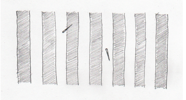
The problem of Buffon’s Needle is described as follows. Imagine that the floor exhibits a pattern of evenly-spaced stripes, all the same width. If you were to drop a needle on the floor, what’s the probability that, when it lands, it crosses from one stripe to another (as opposed to lying entirely within one stripe)? This problem is popular in introductory probability classes, because it can be solved using basic methods in continuous probability.

For the remainder of this post, I assume the stripes have unit width and the needle is one unit long; I leave the general case for your enjoyment. How do we model the location of the needle on the floor? We could model the x and y coordinates of the endpoints of the needle, that would be a complete description using four numbers. Can we do better? Using four numbers, we can describe any line segment of any length in the plane, but we know our needle is exactly one unit long. If we know the location of one point on the needle and the direction it’s pointing then we can infer the end points.

Now let’s suppose we know the x and y coordinates of the midpoint of the needle, as well as its angle of rotation. Can we simplify further? Suppose we choose our coordinates so that the stripes go in the y direction, as in the picture. Because the stripes are parallel, sliding a needle up and down in the y direction won’t change whether it crosses a boundary or not, so to infer whether there is a crossing we only care about the x coordinate and the angle. Moreover, since we don’t care which boundary is crossed, we really on care the x coordinate relative the the stripe that it lives in, which amounts to knowing the fractional part of the x coordinate.

If you believe that, then we can model the position of a needle as a random pair \((x, \theta)\) where \(0 \le x \le 1\) and \(-\pi \le \theta \le \pi\). Intuitively, dropping the needle shouldn’t favor any pair of values over any other, so we put a uniform probability distribution on \((x, \theta)\), namely

$$f(x, \theta) \equiv \frac{1}{2\pi} \text{ on } (0, 1)\times (-\pi, \pi).$$

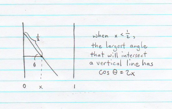
If we can determine the pairs of values \((x, \theta)\) for which a crossing occurs then we solve the problem by integrating \(f\) over that region. Suppose for now that \(x \le 1/2\) is fixed. If we define \(\theta\) to be the angle the needle makes with the negative x-axis, then the largest angle for which the needle crosses a boundary satisfies \(\cos \theta = 2 x\), and since smaller angles correspond to larger cosines, we’ll get a crossing as long as \(\cos \theta \ge 2 x\). We’d also get a crossing if we spun the needle 180 degrees, but we’ll handle that case—along with the case where \(x \ge 1/2\)—using symmetry.

Thus

$$P(\text{crossing}, x \le 1/2, -\pi/2 \le \theta \le \pi/2) = \int_{-\pi/2}^{\pi/2} \int_0^{\cos(\theta)/2} f(x, \theta) dx d\theta = \frac{1}{2\pi}$$

and by symmetry

$$P(\text{crossing}) = 2 P(\text{crossing}, x \le 1/2) = 4 P(\text{crossing}, x \le 1/2, -\pi/2 \le \theta \le \pi/2)$$

hence

$$P(\text{crossing}) = \frac{2}{\pi}.$$

Approximation of \(\pi\)

Since \(\pi\) appears in the solution, we can use repeated needle drops and the Law of Large Numbers to randomly approximate the value of \(\pi\). That is, if \(X_1, \ldots, X_n\) represents an i.i.d. sequence of needle drops where \(X_j\) equals 1 if there is a crossing and 0 otherwise, then

$$\pi \approx \frac{2 n}{\sum_1^n X_j}.$$

I wrote the following R funtion to perform the approximation. Since the goal is to approximate \(\pi\), it seemed like cheating to choose an angle uniformly between \(-\pi\) and \(\pi\), so instead I generate a random direction vector by sampling a bivariate normal distribution and scaling (this is arguably still cheating since \(\pi\) appears in the normal density, but it feels more honest).

BuffonApproximation <- function(n.experiments, n.repetitions) {
  result <- numeric(n.experiments)

  for (i in 1:n.experiments) {
    # generate random position vectors between 0 and 0.5
    x.pos <- runif(n.repetitions, max=0.5)

    # generate random bivariate normal vectors
    x.dir <- rnorm(n.repetitions)
    y.dir <- rnorm(n.repetitions)

    # scale x.dir so it has the distribution of the x-coordinate of a
    # uniformly chosen unit vector
    x.dir <- x.dir / sqrt(x.dir^2 + y.dir^2)

    # now the x-coordinates of the endpoints of the random needle are
    # at x.pos - x.dir and xpos + x.dir. we have a crossing if
    #   x.pos - 0.5 * |x.dir| < 0
    success <- ifelse(x.pos < 0.5 * abs(x.dir), 1, 0)
    result[i] <- 2 * n.repetitions / sum(success)
  }

  result
}

The function performs the approximation n.experiments times, with n.repetitions needle drops in each experiment. Running 200 experiments with 3000 iterations each resulted in a sample mean of 3.147 and a sample standard deviation of 0.045. Not terribly impressive compared to approximations based on power series that were already known in the time of Buffon.