Balanced Sampling
the cube method

I recently read the chapter in Yves Tillé’s Sampling Algorithms about balanced sampling and I thought it would be useful to summarize what I’ve learned. Suppose you want to survey a population about which some data is already known. Specifically, there are auxilliary data points which are known for every individual in the population. A balanced sample is one in which the sample-based estimate for these auxilliary data conform to the true values.

For clarity, call the sampling frame (or universe) \(U\). According to our survey design, individuals \(k \in U\) should be included in the sample with probability \(\pi_k\). The auxilliary data associated with \(k\) will be given by the vector

$$\mathbf x_k = (x_{k1}, \ldots, x_{kp})^T.$$

Let \(S_k\) be a 0-1 indicator variable for \(k\) appearing in our sample. Then the standard Horvitz-Thompson estimator for

$$X = \sum_{k \in U} \mathbf x_k$$

based on our sample would be

$$\hat{X} = \sum_{k \in U} \frac{\mathbf x_k S_k}{\pi_k}.$$

Recall that we assumed the auxilliary data for all individuals is known, so we know \(X\) exactly. One way we might incorporate this knowledge into our sample selection would be to require

$$\hat{X} = X.$$

This is called the balancing equation, and a sample that satisfies the balancing equation is said to be balanced with respect to \(\mathbf x\). Our goal will be to obtain a balanced sample while respecting the inclusion probabilities \(\pi_k\).

Examples

We can cast the fixed-size sample problem in this setting. If \(\sum \pi_k = n\) is an integer, then a sample balanced with respect to \(x_k = \pi_k\) will contain exactly \(n\) individuals since

$$\sum_{k \in U} \frac{x_k S_k}{\pi_k} = \sum_{k \in U} S_k = \sum_{k \in U} \pi_k = n.$$

Note that the first equality follows from the definition \(x_k\) and the second equality is the imposed balancing equation.

Under this scheme, however, the Horvitz-Thompson estimator for the population is random. Instead of constraining the sample size, we might instead constrain our sample so that the sample-estimated population matches the known true population \(N\). This amounts to balancing with respect to \(x_k \equiv 1\) since the balancing equation becomes

$$\sum_{k \in U} \frac{x_k S_k}{\pi_k} = \sum_{k \in U} 1 = N.$$

Geometry of balanced sampling

Now that we’ve defined balanced samples it would be nice if we could get our hands on one. The cube method is an iterative procedure for obtaining samples with the given inclusion probabilities that tries to respect the balance equation. I say “tries” because exact solutions aren’t usually possible. In the example of choosing a fixed-size sample, there are no solutions when \(\sum \pi_k\) is not an integer.

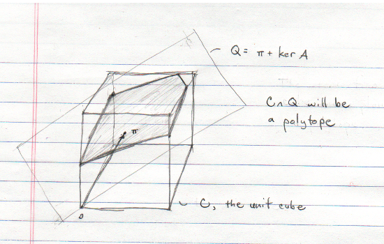
The cube method starts with a geometric interpretation of the balancing equation. Consider

$$\mathbf S = (S_1, \ldots, S_N)$$

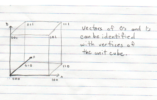
to be a random \(N\)-dimensional vector of 0’s and 1’s. Note that any such vector can be identified with a vertex of the \(N\)-dimensional unit cube \(C\). Let \(p(\mathbf s) = P(\mathbf S = \mathbf s)\). In order to respect the inclusion probabilities \(\pi_k\) we must have

$$\pi = E \mathbf S = \sum_{\mathbf s \in C} p(\mathbf s) \mathbf s$$

where \(\pi = (\pi_1, \ldots, \pi_N)\). This amounts to writing \(\pi\) as a convex combination of cube vertices. Next define \(\check{\mathbf x}_k = \mathbf x_k / \pi_k\) and let \(\mathbf A\) denote the \(p \times N\) matrix with columns \(\check{\mathbf x}_k\). Then we can rewrite the balance equation in matrix notation as

$$\mathbf A \mathbf S = \mathbf A \pi,$$

Moreover, we know from linear algebra that the set of solutions to this equation forms the affine space

$$Q = \pi + \ker \mathbf A.$$

Putting these observations together, we can view a balanced sample as a convex combination of cube vertices that additionally live in \(Q\) and that sum to \(\pi\). As noted above, the balance equation is not always satisfiable and this corresponds geometrically to the fact that the intersection of \(Q\) with the unit cube may not pass through any vertices. As a practical matter, rather than solve for all probabilities \(p(\mathbf s)\) we’ll run a random walk algorithm to set the value of \(\mathbf S\) in such a way that \(E\mathbf S = \pi\).

Taking flight

The cube method operates in two phases. The first is called the flight phase, where we take the aforementioned random walk on \(C\cap Q\). If possible, the random walk may converge to a cube vertex. Otherwise we move on to the landing phase where we “round off” the output of the flight phase. I’m going to focus on the flight phase for the rest of this piece and I’ll come back to the landing phase in a future installment.

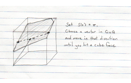
Let’s start with a high-level description. Move to \(\pi\), considered as an \(N\)-dimensional point inside the unit cube (recall that by definition, \(\pi \in Q\)). In the \(n\)th step your current position will be in the intersection of \(Q\) and some number of cube faces (equivalently, you’ll be in \(Q\) and some of your coordinates will be 0 or 1). Choose a direction \(u\), represented as a nonzero \(N\)-dimensional vector, so that if you move a small distance in the direction \(u\) or \(-u\) you won’t leave \(Q\) or any cube faces you belong to. Flip a weighted coin and, depending on the outcome, move in direction \(u\) or \(-u\) until you run into a cube face. This is your new position for the next iteration. Continue to iterate until you can’t choose a direction \(u\) that satisfies the constraints.

A couple notes. First, choosing a direction that leaves you inside \(Q\) amounts to choosing \(u \in \ker \mathbf A\). Second, the coin is weighted so that your expected position at each step is \(\pi\).

Here’s a more formal description of the algorithm.

1. Initialize \(\mathbf S(0) = \pi\).
2. For \(t = 1, 2, \ldots \) until no longer possible, do:
   1. Select \(u(t) \in \ker \mathbf A\) such that \(u_k(t) = 0\) for any \(k\) such that \(\mathbf S_k(t-1) = 0\) or \(1\).
   2. Set \(\lambda^+(t) > 0\) to the maximal value such that \(\mathbf S(t-1) + \lambda^+(t) u(t)\) is in the unit cube. Similarly, set \(\lambda^-(t)\) to the maximal value such that \(\mathbf S(t-1) - \lambda^-(t)u(t)\) is in the unit cube.
   3. With probability \(\lambda^-(t) / (\lambda^+(t) + \lambda^-(t))\) set \(\mathbf S(t) = \mathbf S(t-1) + \lambda^+(t) u(t)\). With the remaining probability set \(\mathbf S(t) = \mathbf S(t-1) - \lambda^-(t) u(t)\).
3. Set \(\mathbf S\) equal to the last \(\mathbf S(t)\) value computed in step 2.

The output of the flight algorithm trivially meets the goals of the previous section. \(Q\) was defined to be the set of points that satisfy the balance equation, and the algorithm ensures that \(\mathbf S \in Q\). Morevover,

$$E \mathbf S(1) = E \mathbf S(0) + \frac{\lambda^-(1)}{\lambda^+(1) + \lambda^-(1)}\lambda^+(1) u(1) - \frac{\lambda^+(1)}{\lambda^+(1) + \lambda^-(1)}\lambda^-(1) u(1) = \pi,$$

hence by induction \(E \mathbf S(t) = \pi\) for all \(t\) and the algorithm samples individuals with the right probabilities.

Computationally, the main work of the flight phase is in sampling from \(\ker \mathbf A\). Tillé gives a variation of the flight phase in which you operate on subsets of columns of \(\mathbf A\), greatly improving efficiency. I won’t go into the details here since the underlying idea is the same, but you should look it up if you choose to write your own implementation.

So far we have generated \(\mathbf S \in C\cap Q\), but there’s no guarantee that the chosen \(\mathbf S\) is a cube vertex (which is required for \(\mathbf S\) to represent a sample). Next time we’ll discuss the landing phase of the cube algorithm which bridges this gap.

You can read part ii of this series here.